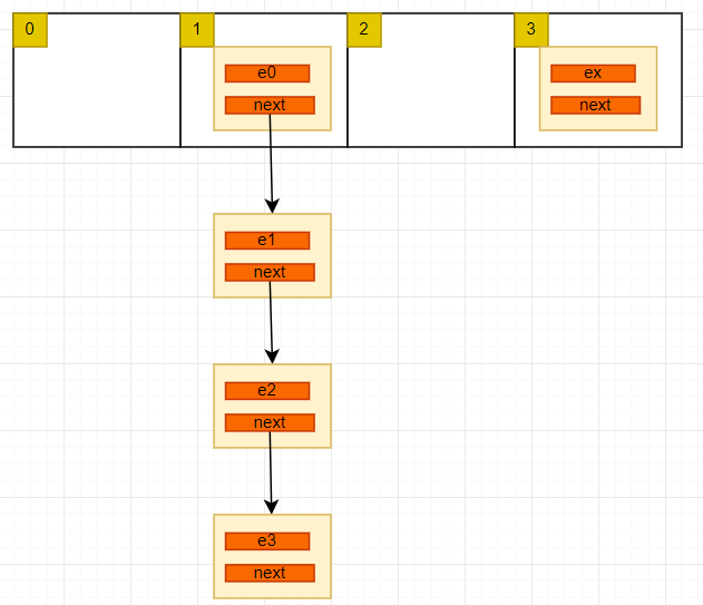
在 JDK 1.8 版本之前,HashMap 底层的数据结构是数组 + 链表,如下图:
在 1.8 及以后是数组 + 链表 + 红黑树
重要的几个变量
- DEFAULT_INITIAL_CAPACITY = 1 « 4; Hash 表默认初始容量
- MAXIMUM_CAPACITY = 1 « 30; 最大 Hash 表容量
- DEFAULT_LOAD_FACTOR = 0.75f;默认加载因子
- TREEIFY_THRESHOLD = 8;链表转红黑树阈值
- UNTREEIFY_THRESHOLD = 6;红黑树转链表阈值
- MIN_TREEIFY_CAPACITY = 64;链表转红黑树时 hash 表最小容量阈值,达不到优先扩容
存放数据
Map <String,Employee> map = new HashMap <> ();
Employee e0 = new Employee("zhangshan");
map.put("zhangshan", e0);
会对 “zhangshan” 进行一次 hash 运算, 把 “zhangshan” 这个字符串映射成一个小于数组长度的整型值。就像下面这样:
int i = hash("zhangshan") 假如 i 等于 1,就会把 e0 构造成一个节点,放入数组下标为 1 的位置。数组存放的是一个节点,该节点有指向下一个节点的指针 next, 如下:
static class Node<K,V> implements Map.Entry<K,V> {
    final int hash;
    final K key;
    V value;
    Node <K,V> next;
}
int i = hash("zhangshan") 把字符串映射成一个整型,不同的字符串可能映射成相同的位置,有下面这种可能:
hash("zhangshan") == hash("lisi")
这就是 hash 碰撞,出现碰撞后,会以链表的方式追加在后面,就形成了上图中的结构。
如何确定 key 在数组中的位置
先看 jdk 1.7 中的实现:
public V put(K key, V value) {
    if (table == EMPTY_TABLE) {
        inflateTable(threshold);
    }
    if (key == null)
        return putForNullKey(value);
    //  获取 key 对应的整型 hash值
    int hash = hash(key);
    // 再将这个hash值转换为小于这个数组的整型值 i,然后将节点插入数组i位置
    int i = indexFor(hash, table.length);
    for (Entry<K,V> e = table[i]; e != null; e = e.next) {
        Object k;
        if (e.hash == hash && ((k = e.key) == key || key.equals(k))) {
            V oldValue = e.value;
            e.value = value;
            e.recordAccess(this);
            return oldValue;
        }
    }

    modCount++;
    addEntry(hash, key, value, i);
    return null;}
其中 hash 方法如下:
final int hash(Object k) {
    int h = hashSeed;
    if (0 != h && k instanceof String) {
        return sun.misc.Hashing.stringHash32((String) k);
    }

    h ^= k.hashCode();

    // This function ensures that hashCodes that differ only by
    // constant multiples at each bit position have a bounded    // number of collisions (approximately 8 at default load factor).
    h ^= (h >>> 20) ^ (h >>> 12);
    return h ^ (h >>> 7) ^ (h >>> 4);
}
我们无需关注实现细节,只需知道这个 hash 方法会返回一个尽量分散的整型值 K. 下面一个关键步骤是如何把 k 转换为一个小于数组长度的值呢? 我们想到最直接的方法是取余运算 %, 即: K % table.length , 是的。这样结果完全没问题,但是性能有问题,在我们常见的 + - * / % 运算中, % 效率是最低的。而 HashMap 作为一个 java 内置的数据结构,会有大量的场景使用。对性能的要求就比较高,自然这里的 indexFor 方法用的不是取余运算,而是 & 运算, 如下:
/**
 * Returns index for hash code h.
 * */
static int indexFor(int h, int length) {
    // assert Integer.bitCount(length) == 1 : "length must be a non-zero power of 2";
    return h & (length-1);
}
这段代码中的注释说。length 必须是 2 的 N 次方,我们来看看这是为什么
& 运算的规则是,同时为 1,结果才是 1,否则是 0,即 1 & 1 == 1 1 & 0 ==0 0 & 0 == 0
而 2 的 N 次方减一,的二进制一定是全为 1,比如 3 , 7 , 15 的二进制是 11 111 1111 。正因为是这种结构, r = h & ( 2 ^ n -1) 的结果 r 一定小于 n, 且 r 取决于 h 的值,由此可以代替取余运算,像这种二进制的 & | ! ^ 运算是最接近计算机底层的,运算速度远远高于 % 运算,我简单测试一下,大约相差 10 倍。
HashMap 的容量
但是要保证上述运算的准确性和效率,其中数组的长度 length 必须是 2 的 N 次方。那么我们在项目中的这种代码:new HashMap<>(13) , 数组的长度是 13 吗? 当然不是,而是以第一个大于 13 且是 2 的 N 次方的数 16, 作为数组的长度。我们先看一下 JDK 1.7 代码:
public V put(K key, V value) {
   //  如果数组为空,初始化数组,而不是在HashMap的构造方法中进行的的
    if (table == EMPTY_TABLE) {
        inflateTable(threshold);
    }
    if (key == null)
        return putForNullKey(value);
    int hash = hash(key);
    int i = indexFor(hash, table.length);
    for (Entry<K,V> e = table[i]; e != null; e = e.next) {
        Object k;
        if (e.hash == hash && ((k = e.key) == key || key.equals(k))) {
            V oldValue = e.value;
            e.value = value;
            e.recordAccess(this);
            return oldValue;
        }
    }

    modCount++;
    addEntry(hash, key, value, i);
    return null;
    }
初始化方法:
private void inflateTable(int toSize) {
// 找到第一个大于等于 toSize 的 2的 N次方的值
int capacity = roundUpToPowerOf2(toSize);
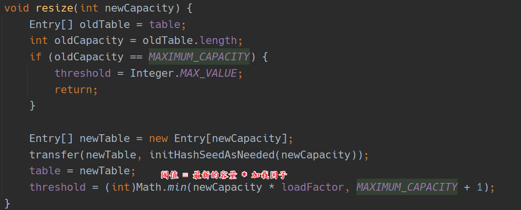
threshold = (int) Math.min(capacity * loadFactor, MAXIMUM_CAPACITY + 1);
table = new Entry[capacity];
initHashSeedAsNeeded(capacity);
}
private static int roundUpToPowerOf2(int number) {
// assert number >= 0 : "number must be non-negative";
return number >= MAXIMUM_CAPACITY
? MAXIMUM_CAPACITY
: (number > 1) ? Integer.highestOneBit((number - 1) << 1) : 1;
}
// 巧妙的通过或运算和位移运算得出第一个大于i的 2 的 N 的数值
public static int highestOneBit(int i) {
// HD, Figure 3-1
i |= (i >> 1);
i |= (i >> 2);
i |= (i >> 4);
i |= (i >> 8);
i |= (i >> 16);
return i - (i >>> 1);
}
关于这个运算原理的讲解参考: https://segmentfault.com/a/1190000039392972
在后续的数组扩容中,新的数组容量也要遵循这个规则,这一点, JDK 1.8 和 1.8 之前的核心实现差不多。
HashMap 的扩容
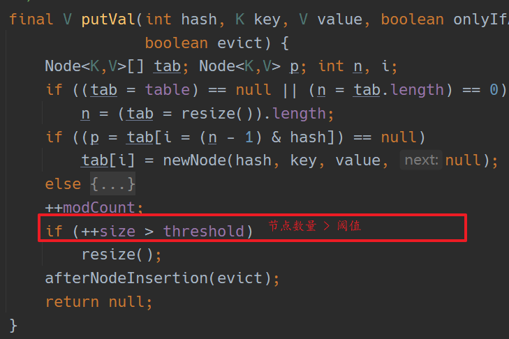
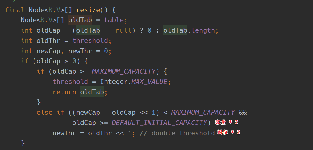
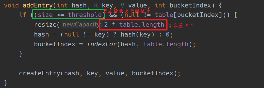
并不是等到节点数量达到容量后才进行的扩容,而是设置了一个阈值,阈值小于等于容量。当节点数量达到阈值后就开始扩容,容量变为原来的 2 倍,在 1.8 之前,阈值 = 容量 * 加载因子。而在 1.8 中,阈值也是原来的 2 倍;如下:
容量和阈值的增长
1.8
1.7
节点的移动方式
在底层数组的扩容方法上,1.8 版本和 1.8 之前的版本相差最大,其中 1.8 之前,HashMap 的扩容在多线程下会产生死循环的问题。
我们先看一下 1.7 版本的扩容 :
1.7版本 节点移动步骤
/**
 * Transfers all entries from current table to newTable.
 */
void transfer(Entry[] newTable, boolean rehash) {
	int newCapacity = newTable.length;
	// 遍历旧数组
	for (Entry<K,V> e : table) {
	    // 遍历链表
		while(null != e) {
			Entry<K,V> next = e.next;
			if (rehash) {
				e.hash = null == e.key ? 0 : hash(e.key);
			}
			// 重新计算当前节点在新数组中的位置
			int i = indexFor(e.hash, newCapacity);
			// 修改节点的指向
			e.next = newTable[i];
			newTable[i] = e;
			// 下一次循环
			e = next;
		}
	}
}
1.7 版本扩容的核心方法只有上面一段,理解起来也不难,主要有下几个步骤:
- 外层遍历数组,假设当前元素: e0
- 内层遍历数组指向的链表,即 e0 为头节点的链表
- 扫描链表的每个节点,重新计算节点的在新数组的位置,将节点移动到新数组中对应的位置,以头插法的方式处理有 Hash 冲突的节点。
一图胜千言:
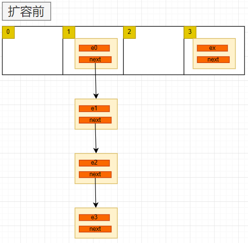
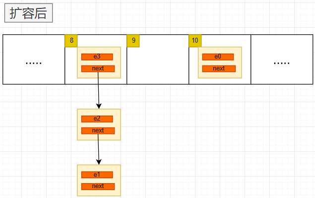
用头插法会导致链表的顺序发生变化。其中每一步不再详解。下面看一下这种扩容方法在多线程下的问题
并发导致的死循环问题
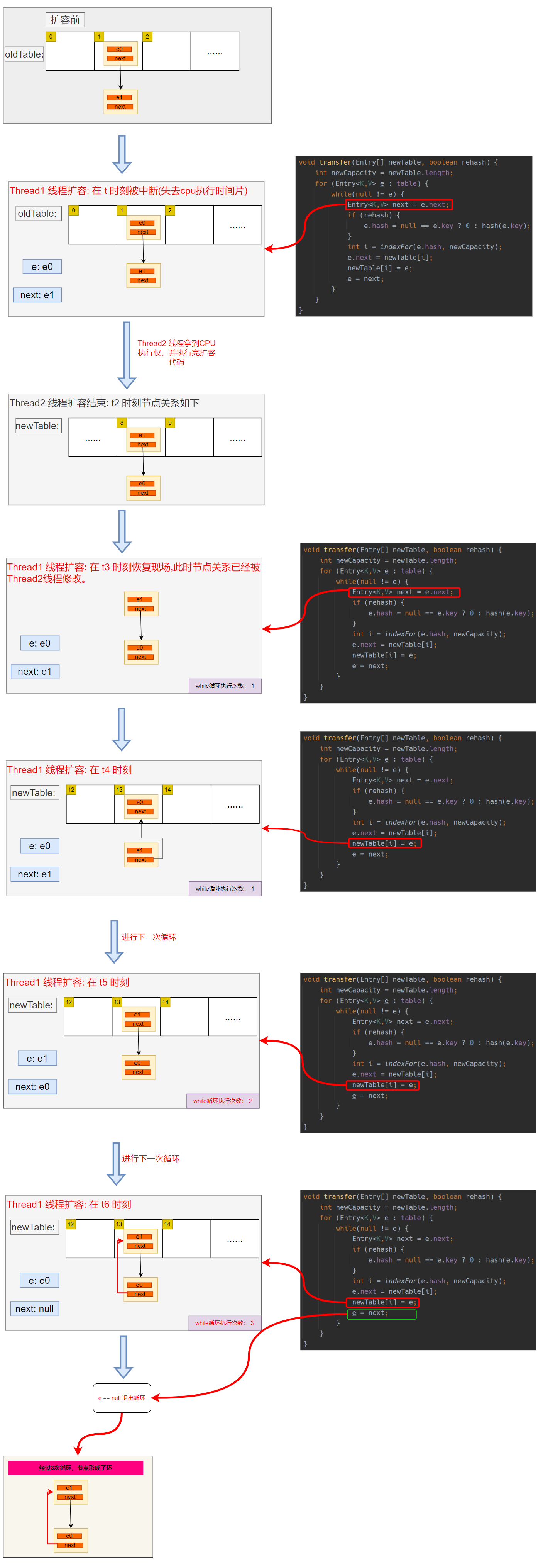
经过几次循环形成了环,Thread1 线程后面在进行 Put 数据时,如果某个key 落在了这个有环节点位置,就会发生死循环。如下:
public V put(K key, V value) {
    if (table == EMPTY_TABLE) {
        inflateTable(threshold);
    }
    if (key == null)
        return putForNullKey(value);
    int hash = hash(key);
    int i = indexFor(hash, table.length);
    // 因为形成了环,导致 e != null 永远成立。死循环
    for (Entry<K,V> e = table[i]; e != null; e = e.next) {
        Object k;
        if (e.hash == hash && ((k = e.key) == key || key.equals(k))) {
            V oldValue = e.value;
            e.value = value;
            e.recordAccess(this);
            return oldValue;
        }
    }

    modCount++;
    addEntry(hash, key, value, i);
    return null;
}
下面我们对比看一下 1.8 版本是如何解决这个问题的。
1.8版本 节点移动步骤
在1.8版本中仍保留了 数组+链表的结构,只有当HashMap中的容量大于某个值时,才会把链表转换为红黑树,提高检索效率。现在我们只关注扩容部分。
扩容的关键代码:
final Node<K,V>[] resize() {
    Node<K,V>[] oldTab = table;
    int oldCap = (oldTab == null) ? 0 : oldTab.length;
    int oldThr = threshold;
    int newCap, newThr = 0;
    if (oldCap > 0) {
        if (oldCap >= MAXIMUM_CAPACITY) {
            threshold = Integer.MAX_VALUE;
            return oldTab;
        }
        else if ((newCap = oldCap << 1) < MAXIMUM_CAPACITY &&
                 oldCap >= DEFAULT_INITIAL_CAPACITY)
            newThr = oldThr << 1; // double threshold
    }
    else if (oldThr > 0) // initial capacity was placed in threshold
        newCap = oldThr;
    else {               // zero initial threshold signifies using defaults
        newCap = DEFAULT_INITIAL_CAPACITY;
        newThr = (int)(DEFAULT_LOAD_FACTOR * DEFAULT_INITIAL_CAPACITY);
    }
    if (newThr == 0) {
        float ft = (float)newCap * loadFactor;
        newThr = (newCap < MAXIMUM_CAPACITY && ft < (float)MAXIMUM_CAPACITY ?
                  (int)ft : Integer.MAX_VALUE);
    }
    threshold = newThr;
    @SuppressWarnings({"rawtypes","unchecked"})
    Node<K,V>[] newTab = (Node<K,V>[])new Node[newCap];
    table = newTab;
    if (oldTab != null) {
        for (int j = 0; j < oldCap; ++j) {
            Node<K,V> e;
            if ((e = oldTab[j]) != null) {
                oldTab[j] = null;
                if (e.next == null)
                    newTab[e.hash & (newCap - 1)] = e;
                else if (e instanceof TreeNode)
                    ((TreeNode<K,V>)e).split(this, newTab, j, oldCap);
                else { // preserve order
                   // 定义了四个指针
                    Node<K,V> loHead = null, loTail = null;
                    Node<K,V> hiHead = null, hiTail = null;
                    Node<K,V> next;

                    // 开始扩容
                    do {
                        next = e.next;
                        // 节点的hash值与 旧数组的容量相与,oldCap 是2的N次方
                        // 一个数和 2的N次方相与时,结果只能是0或 oldCap
                        if ((e.hash & oldCap) == 0) {
                            if (loTail == null)
                                // 指定头指针的位置
                                loHead = e;
                            else
                                // 前一个指针的后继节点是当前节点
                                loTail.next = e;
                            // 尾指针锚定当前节点
                            loTail = e;
                        }
                        else {
                            if (hiTail == null)
                                hiHead = e;
                            else
                                hiTail.next = e;
                             hiTail = e;
                        }
                    } while ((e = next) != null);
                    // 低位节点的下标不变
                    if (loTail != null) {
                        loTail.next = null;
                        newTab[j] = loHead;
                    }
                    // 高位节点下标增加 oldCap
                    if (hiTail != null) {
                        hiTail.next = null;
                        newTab[j + oldCap] = hiHead;
                    }
                }
            }
        }
    }
    return newTab;
}
这里定义了四个指针,将某个链表分为两部分,链表节点和数组长度相与的结果作为分隔,等于0的放在以loHead为头节点的链表中,等1的放在以hiHead为头节点的链表中。如下图:
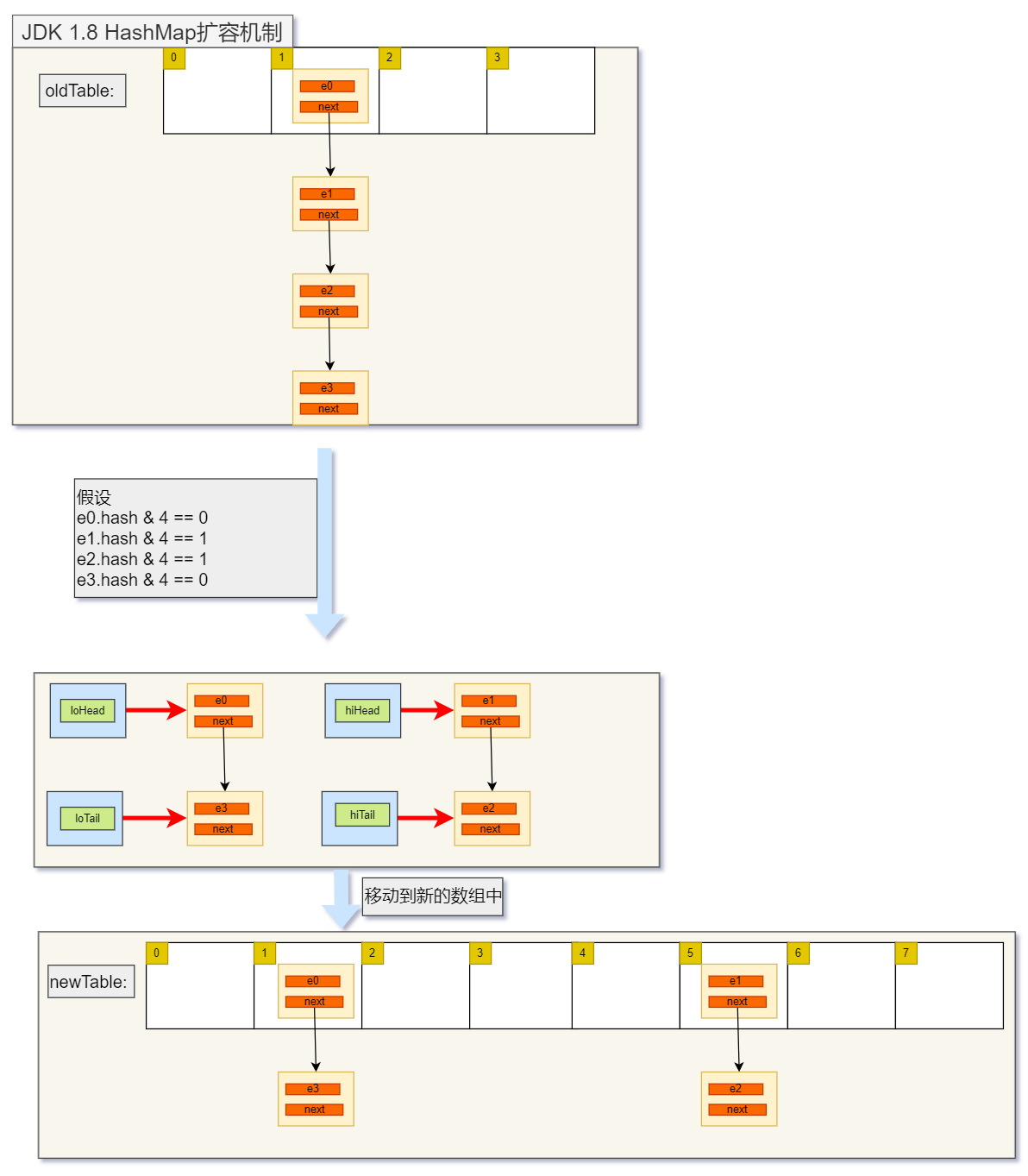
如上所示。这种移动方式没有改变节点关系的方向,所以并发之下也没有问题
扩容因子为什么是0.75
1.8版本链表与红黑树的转换
- 链表长度 > 8
- 容量 > 64
- 性能提升的不是很高,在大量数据下,可能会提升5% ~10%, 数据量不大时。没有什么区别
- 红黑树